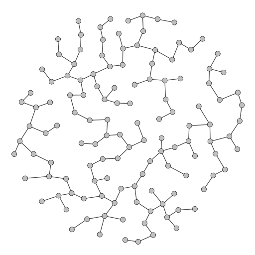
Kirchhoff’s Matrix Tree Theorem for Counting Spanning Trees — A Proof for Beginners

Rectilinear minimum spanning tree (source: Rocchini)

In this post, we provide a proof of Kirchhoff’s Matrix Tree theorem [1] which is quite beautiful in our biased opinion. This is a 160-year-old theorem which connects several fundamental concepts of matrix analysis and graph theory (e.g., eigenvalues, determinants, cofactor/minor, Laplacian matrix, incidence matrix, connectedness, graphs, and trees etc.). There are already many expository articles/proof sketches/proofs of this theorem (for example, see [4-6, 8,9]). Here we compile yet-another-expository-article and present arguments in a way which should be accessible to the beginners.

Statement

Suppose $L$ is the Laplacian of a connected simple graph $G$ with $n$ vertices. Then the number of spanning trees in $G$ , denoted by $t(G)$ , is the following:

$t(G)=\frac{1}{n} \times \{$ the product of all non-zero eigenvalues of $L\ \}$ .

Before we proceed to the proof, let us give some definitions. We assume that some elementary concepts of linear algebra (e.g., rank, determinant, eigenvalue/eigenvector, minor/cofactor, etc.) are known to the reader. However, we use some known “facts” that we do not prove in this article.

The proof has two main parts:

Part 1: We prove that the number of spanning trees in a connected simple graph is equal to any cofactor of the Laplacian matrix of that graph. This is the heart of the theorem/proof.

Part 2: Next we use standard linear algebra results to relate the cofactor of any matrix and its eigenvalues. Since the matrix we use is the graph Laplacian, it readily relates the eigenvalues (of the Laplacian) with the number of spanning trees (using the result from previous part). This part can be found in any standard text in matrix analysis; for example: see Theorem 1.2.12, and Definitions 1.2.5 and 1.2.9 in the Horn and Johnson book [7].

Now we mention some preliminaries.

Preliminaries

(For concepts that are considered basics in linear algebra, we provide hyperlinks to detailed exposition.)

Let $G$ be a graph on $n$ vertices and $m$ edges. $A$ is the $n\times n$ adjacency matrix of $G$ with zeros in the main diagonal and the entry $A(i,j)=A(j,i)=1$ whenever the edge $(i,j)$ exists, and $A(i,j)=A(j,i)=0$ when the edge $(i,j)$ does not exist.

Let $D$ be the $n\times n$ diagonal matrix whose $(i,i)$ entry is the degree of the vertex $i$ . The combinatorial Laplacian, or simply Laplacian, is the $n\times n$ matrix $L=D-A$ . Note that sum of all entries in any row of $L$ is $0$ (why?); that is why the constant vector $[1 1 \cdots 1]^T$ is an eigenvector of $L$ with eigenvalue $0$ . Since all eigenvalues of $L$ are non-negative, $0$ must be the smallest eigenvalue of $L$ .

Let $B$ be the $n\times m$ incidence matrix where columns correspond to edges and rows correspond to vertices, and any column $b_e$ , corresponding to the edge $e=(i,j)$ ), contains zeros at all rows except at two positions: $b_e(i)=1$ and $b_e(j)=-1$ . Note that $L$ can be written as the “square” of the incidence matrix; that is, $L=BB^T$ .

Let $C_{kk}$ be the cofactor of the $k^\text{th}$ diagonal element of a square matrix. Let $[L]_{k,k}$ be the $k^\text{th}$ principal minor of any square matrix $L$ .

Now let us mention some facts of which we will not present proofs.

Some Facts from Matrix Analysis

Fact F1. Let $\widetilde{B}_k$ be the $(n-1)\times m$ submatrix obtained from the $n\times m$ incidence matrix $B$ by removing its $k^\text{th}$ row. Then, the cofactor of the $k^\text{th}$ diagonal element of the Laplacian $L$ is the following:

$C_{kk}=det(\widetilde{B}_k {\widetilde{B}_k}^T )$

Proof: See the “Omitted Proofs” section.

Fact F2. Cauchy-Binet formula for determinant, which can compute the determinant of the product of two matrices, say $det(A,B)$ , from the determinants of the submatrices of $A$ and $B$ .

Fact F3. (Unused)

Fact F4. The product of all non-zero eigenvalues of the combinatorial Laplacian $L$ is equal to the sum of all principal minors of $L$ . That is,

$\lambda_2\lambda_3\lambda_4\cdots \lambda_n=\sum_{k=1}^n{[L]_{k,k}}$

where $[L]_{k,k}$ is the $k^\text{th}$ principal minor of $L$ .

Proof: See the “Omitted Proofs” section below.

F5. Diagonal cofactors of an $n\times n$ square matrix are equal to corresponding principal minors. That is,

$C_{kk}=[L]_{k,k} \ \text{for }1\leq k\leq n$ .

Proof(of F5): Same as the proof sketch of F4.

Now we will establish some relationship between the incidence matrix $B$ and the connectedness of $G$ .

Rank of submatrices of the Incidence Matrix $B$

Note that each column of the incidence matrix has exactly one $1$ and one $-1$ . Let us define the row sum of a column of any matrix as the sum of all entries in that column. Similarly, let the row sum of a matrix be the sum of all its entries. Now note that if $G$ is connected, each column of the incidence matrix $B$ contains exactly two non-zero entries $1$ and $-1$ , and thus row sum at each column is zero. Now, this implies that the sum of all row vectors of $B$ is the zero-vector and hence any row can be expressed as a linear combination of all other rows. Therefore, rows of $B$ are linearly dependent, which means the rank of $B$ must be smaller than $n$ . Thus we have the following claim:

Proposition P1. If $G$ is connected and $B_G$ is its incidence matrix, then $rank(B_G) \leq n-1$ .

Now consider a subgraph $H$ of $G$ on $k < n$ vertices such that $rank(B_H)=k$ . This means, all rows of $B_H$ are linearly independent, and thus there is at least one column in $B_H$ for which the row-sum is not zero. This implies that there is at least one edge $e=(u,v)$ which connects a vertex in $H$ to a vertex outside $H$ . In other words, $H$ cannot be a connected component of $G$ . Therefore, we have the following claim:

Proposition P2. If the rank of the incidence matrix $B_H$ is $n-1$ for a $(n-1)$ -vertex subgraph $H$ of $G$ , then $G$ is connected.

Now we will prove an important fact about the determinant of any $(n-1)\times (n-1)$ square submatrix of $B$ .

Lemma L0. The determinant of any $(n-1)\times (n-1)$ square submatrix of $B$ is either 0 or $\pm 1$ .

Proof: See the “Omitted Proofs” section.

Rank of $B$ and Connectedness of $G$

Let $\widetilde{B}$ be a non-empty submatrix obtained from $B$ by removing exactly one row from $B$ . Note that at least one column of $\widetilde{B}$ will have non-zero row sum. Therefore, rows of $\widetilde{B}$ will be linearly independent, and $rank(\widetilde{B})$ must be greater than or equal to the number of rows of $\widetilde{B}$ . Since $\widetilde{B}$ has $n-1$ rows, it follows that $rank(\widetilde{B}) \geq n-1$ .

However, the rank of the incidence matrix $B$ must be greater than or equal to the rank of any row-subset of $B$ , such as $\widetilde{B}$ . Since the largest row-subset of $B$ will have $(n-1)$ rows, we can have the following claim:

Proposition P3. If $G$ is connected and $B$ is its incidence matrix, then $rank(B) \geq n-1$ .

Now we will prove the following lemma.

Lemma L1. (Rank of the Incidence matrix of a connected graph) Let $B$ be the incidence matrix of graph $G$ . Then, $G$ is connected $\Leftrightarrow rank(B)=n-1$ .

Proof: See the “Omitted Proofs” section below.

The Connection between Spanning Trees and the Incidence Matrix

The subgraph $T(V,\widetilde{E})$ will be a spanning tree of the graph $G(V,E)$ if it has the following properties:

$T$ has $n$ vertices and $n-1$ edges.
$T$ is connected.
The incidence matrix $B_T$ , whose columns correspond to the $n-1$ edges of $T$ , has $n$ rows.

Let us consider $B_T$ , which is a $n\times (n-1)$ matrix. Since $T$ is connected, there will be no row with all zero entries, and according to Lemma L1 we know that $rank(B_T)=n-1$ . This means any collection of $n-1$ rows of $B_T$ are linearly independent. Consequently, any row-subset $\widetilde{B}$ of $B_T$ containing $n-1$ rows (and all $n-1$ columns) will have rank $n-1$ . Now, since $\widetilde{B}$ is a square matrix with $n-1$ rows and $n-1$ columns with rank $n-1$ , it follows that $det(\widetilde{B}) \neq 0$ . Therefore we have proved the following lemma:

Lemma L2. (Determinant of an order- $(n-1)$ square submatrix of $B_T$ )
If $B_T$ is the incidence matrix of a spanning tree $T$ of $G$ , every $(n-1)\times (n-1)$ square submatrix of $B_T$ is non-singular.

The above Lemma also leads us to the following elegant result.

Lemma L3. (Spanning tree of $G$ and incidence matrix $B$ ) Let $G$ be a graph with $n$ vertices, and let $B$ be its incidence matrix. Let $H$ be a subgraph of $G$ with $n-1$ edges, and let $B_H$ be its incidence matrix. Then, $H$ is a spanning tree of $G \Leftrightarrow$ every $(n-1) \times (n-1)$ square submatrix of $B_H$ is non-singular.

Proof: See the “Omitted Proofs” section below.

We can readily get the following corollary.

Corollary C1.
Each non-singular $(n-1)\times (n-1)$ square submatrix of $B$ corresponds to a spanning tree of $G$ induced by its columns.

Proof: See the “Omitted Proofs” section.

The above corollary leads us to the following simple yet beautiful result.

Lemma L4. (Number of spanning tree and the incidence matrix $B$ )
Let $\widetilde{B}_k$ be a submatrix of $B$ derived by removing the $k^\text{th}$ row from $B$ . Thus $\widetilde{B}_k$ has $n-1$ rows and $m$ columns. Then, the number of spanning trees in $G$ , denoted by $t(G)$ , is equal to the number of non-singular $(n-1)\times (n-1)$ submatrices of $\widetilde{B}_k$ .

Proof: See the “Omitted Proofs” section below.

Let us call $\widetilde{B}_k$ the Reduced Incidence Matrix, derived by removing the $k^\text{th}$ row from $B$ . Thus the question of computing $t(G)$ , the number of spanning trees in $G$ , is equivalent to computing the number of non-singular $(n-1)\times (n-1)$ square submatrices of the reduced incidence matrix $\widetilde{B}_k$ .

Now we can proceed to the proof of the main theorem.

Proof of the Main Theorem

First, let us briefly state what we are going to prove. Let $0=\lambda_1 \leq \lambda_2 \leq \lambda_3 \leq\cdots \leq \lambda_n$ be the $n$ eigenvalues (counting multiplicities) of the combinatorial Laplacian $L$ of the graph $G$ . We want to prove that

$t(G)=\frac{1}{n}\times \prod_{k=2}^n{\lambda}_k$ .

We will proceed as follows.

Step 1: (Submatrix $P$ from $B$ ) Let $P$ be an $(n-1)\times m$ submatrix of the incidence matrix $B$ by deleting the $k^\text{th}$ row of $B$ . Using Fact F1, we see that

$C_{kk}=det(PP^T)$ .

Note that $P$ has $n-1$ rows and $m$ columns. We want

Step 2: (Square submatrices of $P$ of order $n-1$ ) Now we will build all $(n-1)\times (n-1)$ submatrices from $P$ as follows. Let $s$ be any ordered sequence of $n-1$ integers picked from $1,2,3,\cdots, m$ such that $s_i < s_{i+1}$ . Let $S$ be the set of all such sequences $s$ . Now, given a particular sequence $s$ , let $P_s$ be the $(n-1)\times (n-1)$ submatrix of $P$ obtained by keeping only those columns from $P$ whose index are in $s$ .

Step 3: (Apply Fact F2) We want to evaluate the determinant from Step 1 using Cauchy-Binet formula, as follows:

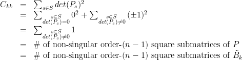
$\begin{array}{rcl}C_{kk}&=&det(PP^T)\\&=&\sum_{s\in S}{det(P_s)\times det(P_s^T)}\\&=&\sum_{s\in S}{det(P_s)^2}\ \ \text{since }det(P_s)=det(P_s^T)\\\end{array}$

Step 4: (Apply Lemma L0) $P_s$ must be either $0$ or $\pm 1$ , and hence the above equation becomes the following:

$\begin{array}{rcl}C_{kk}&=&\sum_{s\in S}{det(P_s)^2}\\&=&\sum_{\substack{s\in S\\det(P_s)=0}}{0^2}+\sum_{\substack{s\in S\\det(P_s)\neq 0}}{(\pm 1)^2}\\&=&\sum_{\substack{s\in S\\det(P_s) \neq 0}}{1}\\&=&\text{\# of non-singular order-}(n-1)\text{ square submatrices of }P\\&=&\text{\# of non-singular order-}(n-1)\text{ square submatrices of }\tilde{B}_k\end{array}$

Step 5: (Apply Lemma L4) By Lemma L4, the number of spanning trees in $G$ is the same as the number of non-singular $(n-1)\times (n-1)$ square submatrices of $B$ . Therefore, the above equation becomes

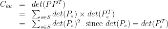
$C_{kk}=\text{\# number of spanning trees of }G=t(G)$ .

Step 6: Note that the value of $t(G)$ does not depend on $k$ , and thus each diagonal cofactor of the combinatorial Laplacian $L$ is equal to $t(G)$ .

$t(G)=C_{11}=C_{22}=C_{33}=\cdots = C_{nn}$ .

Step 7: (Use Facts F4, F5) Restating Fact F4, we have,

$\begin{array}{rcl}\lambda_2\lambda_3\lambda_4\cdots \lambda_n&=&\sum_{k=1}^n{[L]_{k,k}}\ \ \text{by F4}\\&=&\sum_{k=1}^n{C_{k,k}}\ \ \text{by F5}\\&=&n\times t(G)\ \ \text{by Step 6}\\\end{array}$

Thus, we have proved Kirchoff’s Matrix-Tree theorem.

$\square$

Omitted Proofs

$C_{kk}=det(\widetilde{B}_k {\widetilde{B}_k}^T )$

Proof sketch (of F1): First note that for unweighted graphs, $L=BB^T$ and hence, every $(i,j)$ entry of $L$ comes from the dot product of the $i^\text{th}$ row and $j^\text{th}$ column of $B$ . Now, the $(n-1)\times (n-1)$ matrix $\widetilde{B}_k\widetilde{B}_k^T$ will not have any contribution from the $k^\text{th}$ row and $k^\text{th}$ column of $B$ . This is exactly what happens when computing $C_{kk}$ : First we take the $k^\text{th}$ principal minor by removing the $k^\text{th}$ row/column from $B$ and then take determinant. (The sign of $C_{kk}$ will be $(-1)^{k+k}=(-1)^{2k}$ , which is positive.) $\square$

Fact F4. The product of all non-zero eigenvalues of the combinatorial Laplacian $L$ is equal to the sum of all principal minors of $L$ . That is,

$\lambda_2\lambda_3\lambda_4\cdots \lambda_n=\sum_{k=1}^n{[L]_{k,k}}$

where $[L]_{k,k}$ is the $k^\text{th}$ principal minor of $L$ .

Proof sketch (of F4): Since eigenvalues are solutions to the characterstic polynomial $\chi(M)$ of a square matrix $M$ , they can be related to the coefficients of $\chi(M)$ by using elementary symmetric polynomials. Next, the coefficients of $\chi(M)$ can be expressed as the sum of principal minors of $M$ . Details can be found in any standard matrix analysis textbook, e.g., Chapter 0 of [7]. $\square$

Lemma L0. The determinant of any $(n-1)\times (n-1)$ square submatrix of $B$ is either 0 or $\pm 1$ .

The following proof is taken from the Masters Thesis of Boomen [6].

Proof: The proof is by induction.

(Base case) First observe that only two nonzero entries appear at each column of $B$ , and one of them is $1$ and the other is $-1$ . Now consider any $2\times 2$ submatrices of $B$ where each entry is either 0 or $\pm 1$ and the nonzero entries in a column are different. It can be checked that the value of the determinant of this submatrix can only be one of $\{0,\pm 1\}$ . This forms the basis of our induction.

(Induction hypothesis) Assume that the determinant of every square submatrix of $B$ of order smaller than $n-1$ is either 0 or $\pm 1$ .

(Induction) Suppose $\widetilde{B}$ be a $(n-1)\times (n-1)$ square submatrix of $B$ . We want to show that the $det(\widetilde{B}) \in \{0, \pm 1\}$ .

Think about Laplace expansion of the determinant of $\widetilde{B}$ . There can be only three cases:

Case 1: If there is any row/column with all zeros, $det(\widetilde{B}=0$ and we are done.
Case 2: If any row/column of $\widetilde{B}$ contains exactly one nonzero entry ( $\pm 1$ ), we expand $det(\widetilde{B})$ along that row/column (which will have only one cofactor) and by applying the inductive hypothesis, the result is $\pm 1 \times \{0,\pm 1\}$ which is either 0 or $\pm 1$ , and we are done.
Case 3: If all columns of $\widetilde{B}$ contain exactly two nonzero entries (one 1 and the other -1), then if we add all rows the sum will be the zero vector. Hence $rank(\widetilde{B})=0$ and therefore $det(\widetilde{B})=0$ , and we are done.

$\square$

Lemma L1. (Rank of the Incidence matrix of a connected graph) Let $B$ be the incidence matrix of graph $G$ . Then, $G$ is connected $\Leftrightarrow rank(B)=n-1$ .

Proof:
(The $\Rightarrow$ part.) From Propositions 1 and 3, we see that if $G$ is connected, then $(n-1) \leq rank(B) \leq (n-1)$ , which means $rank(B) = n-1$ .

(The $\Leftarrow$ part.) It given that $rank(B)=n-1$ . Therefore, there exists a $(n-1)\times m$ submatrix of $B$ , call it $\widetilde{B}$ , whose rank is $n-1$ . Suppose $\widetilde{B}$ is the incidence matrix of the subgraph $H(\widetilde{V},\widetilde{E})$ of $G$ on $n-1$ vertices. Since $rank(\widetilde{B})=\#\text{rows}(\widetilde{B})$ , we can apply Proposition 4 and hence $G$ is connected. $\square$

Proof:
(The $\Rightarrow$ part.) Apply Lemma L2.
(The $\Leftarrow$ part.) If every $(n-1) \times (n-1)$ submatrix $\widetilde{B}$ of the $n \times (n-1)$ matrix $B$ is non-singular, it implies that $rank(\widetilde{B})= n-1=\#\text{rows}(\widetilde{B})$ . Therefore, applying Proposition 2 we can see that $H$ is connected. Since $H$ has exactly $n-1$ edges on $n$ vertices, $H$ must be a tree. Hence, $H$ is a spanning tree. $\square$

Corollary C1.
Each non-singular $(n-1)\times (n-1)$ square submatrix of $B$ corresponds to a spanning tree of $G$ induced by its columns.

Proof:
Let $G(V,E)$ be a connected graph. Let $Q$ be a non-singular $(n-1)\times (n-1)$ square submatrix of $B$ and let $G_Q(V_Q,E_Q)$ be the subgraph for which $Q$ is the incidence matrix. Assume, without loss of generality, that $V_Q=\{v_1,v_2,\cdots,v_{n-1}\}$ . Since $rank(Q)=n-1$ (because it is non-singular), at least one of its columns will have non-zero row-sum and thus one of its edges must be incident to the vertex $u$ such that $u \in V \setminus V_Q$ . Thus the subgraph $T(V_Q \cup \{u\}, E_Q)$ is connected, has $n$ vertices and $n-1$ edges, and thus it is a spanning tree of $G$ and has the same edges that correspond to the columns of $Q$ . $\square$

Proof:
By Corollary C1 each non-singular $(n-1)\times (n-1)$ submatrix $Q$ of $\widetilde{B}_k$ corresponds to a spanning tree. However, since $\widetilde{B}_k$ has $n-1$ rows, each $Q$ has a different set of edges, and thus corresponds to a different spanning tree. Therefore the number of spanning trees in $G$ is the same as the number of non-singular submatrices of $\widetilde{B}_{k}$ with dimension $(n-1)\times (n-1)$ . $\square$

References

[1] Kirchhoff, G. Über die Auflösung der Gleichungen, auf welche man bei der untersuchung der linearen verteilung galvanischer Ströme geführt wird. Ann. Phys. Chem. 72, 497-508, 1847.

[2] Deo, N., Graph theory wity applications to Engineering and Computer Science, Prentice Hall, Englewood Clis, New Jersey, 1974.

[3] Lankaster, P., Tismenetsky, M., Theory of matrices : with applications, 2nd edition, Academic Press, 1985.

[4] Butler, S. K., Eigenvalues and Structures of Graphs, PhD Dissertation, University of California at San Diego, 1-9, 2008.

[5] Brualdi, R. A., The Mutually Beneficial Relationship of Graphs and Matrices, American Mathematical Society, 21-22, 2011.

[6] Boomen, J., The Matrix Tree Theorem, Masters thesis, Radboud Universiteit Nijmegen, Netherlands, 2007.

[7] Horn, Roger A., and Charles R. Johnson. “Matrix Analysis. 1985.” Cambridge, Cambridge.

[8] Srivastava, Nikhil. Matrix Tree Theorems (Lecture Notes). http://www.cs.yale.edu/homes/spielman/561/2009/lect18-09.pdf

[9] Oveis Gharan, Shayan. Random Spanning Trees (Lecture Notes). https://homes.cs.washington.edu/~shayan/courses/cse599/adv-approx-1.pdf

7 thoughts on “Kirchhoff’s Matrix Tree Theorem for Counting Spanning Trees — A Proof for Beginners”

Deli Zhang says:

April 10, 2015 at 11:13 am

Reblogged this on Deli Zhang.

Deli Zhang says:

April 10, 2015 at 11:19 am

Hi Saad, you must be interesting in my article — The Formula for the Equivalent Resistance of Complex Resistance Network
It’s a typical application of Metrix-Tree theorem, I just can say wanderful. Please see https://zhangdeli.wordpress.com/

Phuong Hoa says:

May 16, 2016 at 5:00 am

Helo, I’m Phương Hoa. I’m come from Viet Nam. And I can’t find and download: [7] Horn, Roger A., and Charles R. Johnson. “Matrix Analysis. 1985.” Cambridge, Cambridge. So can you proof F4 and F5? It’s very important for me. Please!

Tobias Harvey says:

January 15, 2017 at 11:12 am

I am fairly certain that there is a typo here, “Let us consider B_T, which is a n\times m matrix. Since T is connected, according to Lemma L1 we know that rank(B_T)=n-1, which means the row-sum of B_T is not zero, and hence any set of n-1 rows of B_T are linearly independent. ” B_T is connected without an edge leading out of it (every column sums to zero), therefore it does row reduce to zero, but does still have n-1 linearly independent vectors, just not n linearly independent vectors. Let my know if I have misinterpreted what B_T is.

Also is B_T n x n-1 or n x m, or n x m where m = n – 1. seemed a little unclear.

1. saad0105050 says:
  
  January 31, 2017 at 2:44 pm
  
  Indeed, $B_T$ has dimension $n\times (n-1)$ . I have fixed that. Moreover, you are right about the row-sum of $B_T$ , it is zero. What I wrote was incorrect. I updated the lines as follows:
  “according to Lemma L1 we know that $rank(B_T)=n-1$ , which means any collection of $n-1$ rows of $B_T$ are linearly independent.”
  
  Sorry for the late reply.
  
Tobias Harvey says:

January 15, 2017 at 11:17 am

But this is a really cool proof thank you!

1. saad0105050 says:
  
  January 31, 2017 at 3:03 pm
  
  Thanks. But it is not “my” proof: I collected the pieces together from other proofs. Thanks for your comments.

Kirchhoff’s Matrix Tree Theorem for Counting Spanning Trees — A Proof for Beginners

Statement

Preliminaries

Some Facts from Matrix Analysis

Rank of submatrices of the Incidence Matrix $B$

Rank of $B$ and Connectedness of $G$

The Connection between Spanning Trees and the Incidence Matrix

Proof of the Main Theorem

Omitted Proofs

References

Published by saad0105050

7 thoughts on “Kirchhoff’s Matrix Tree Theorem for Counting Spanning Trees — A Proof for Beginners”

Leave a comment Cancel reply

Statement

Preliminaries

Some Facts from Matrix Analysis

Rank of submatrices of the Incidence Matrix

Rank of and Connectedness of

The Connection between Spanning Trees and the Incidence Matrix

Proof of the Main Theorem

Omitted Proofs

References

Share this:

Related

Published by saad0105050

7 thoughts on “Kirchhoff’s Matrix Tree Theorem for Counting Spanning Trees — A Proof for Beginners”

Leave a comment Cancel reply

Rank of submatrices of the Incidence Matrix $B$

Rank of $B$ and Connectedness of $G$