Fractional Moments of the Geometric Distribution

In one of my papers, I needed an upper bound on the fractional moments of the geometric distribution. The integer moments have a nice-looking upper bound involving factorials. In addition, Mathematica showed that the same upper bound holds for fractional moments once we use Gamma function instead of factorials. The problem was, I could not prove it. Worse, I could not find a proof after much looking on the Internet.

This post contains a proof that for any real $\lambda > 1$ , the $\lambda$ th moment of a geometric random variable with success probability $\displaystyle p \geq 1/2$ is at most $\displaystyle \Gamma(\lambda + 1)/p^\lambda$ .

Continue reading “Fractional Moments of the Geometric Distribution” →

Our Paper on Realizing a Graph on Random Points

Our paper, titled How to Realize a Graph on Random Points, has been accepted at CCCG (Canadian Conference on Computational Geometry) 2019. I’ll write more about it in future posts.

Abstract:

Continue reading “Our Paper on Realizing a Graph on Random Points” →

Random Walk on Integers

Unbiased Random Walks (source:Wikipedia) — Unbiased Random Walks

Imagine that a particle is walking in a two-dimensional space, starting at the origin $(0, 0)$ . At every time-step (or “epoch”) $n = 0, 1, 2, 3, \cdots$ it takes a $\pm 1$ vertical step. At every step, the particle either moves up by $+1$ , or down by $-1$ . This walk is “unbiased” in the sense that the up/down steps are equiprobable.

In this post, we will discuss some natural questions about this “unbiased” or “simple” random walk. For example, how long will it take for the particle to return to zero? What is the probability that it will ever reach +1? When will it touch $a$ for the first time? Contents of this post are a summary of the Chapter “Random Walks” from the awesome “Introduction to Probability” (Volume I) by William Feller. Also, this is an excellent reference.

Edit: the Biased Case. The biased walk follows

$\displaystyle p:=\Pr[ \text{down}]\, ,\qquad q:=\Pr[ \text{up} ]\, ,\qquad p + q = 1$ .

The lazy walk follows

$\displaystyle p:=\Pr[ \text{down}]\, ,\qquad q:=\Pr[ \text{up} ]\, , \qquad \Pr[stay] = r\, ,\qquad p + q = 1$ .

In the exposition, we’ll first state the unbiased case and when appropriate, follow it up with the biased case.

Continue reading “Random Walk on Integers” →

Characterizing the Adversarial Grinding Power in a Proof-of-Stake Blockchain Protocol

[Contents of this post are based on an ongoing discussion with Alex Russell and Aggelos Kiayias. It contains potentially unpublished material.]

In a proof-of-stake blockchain protocol such as Ouroboros, at most half of the users are dishonest. While an honest user always extends the longest available blockchain, the dishonest users try to fool him into extending a manipulated blockchain. Here, the user who is allowed to issue a block at any time-slot is called the “slot leader.” As it happens, a number of future slot leaders are computed in advance using the random values present in the blocks. Although counterintuitive, such a scheme ensures that if the adversary does not control more than half the users now, it is very unlikely that he cannot control more than half the slot leaders. The time-slots are divided into “epochs” of length $R$ .

Continue reading “Characterizing the Adversarial Grinding Power in a Proof-of-Stake Blockchain Protocol” →

Forkable Strings are Rare

In a blockchain protocol such as Bitcoin, the users see the world as a sequence of states. A simple yet functional view of this world, for the purpose of analysis, is a Boolean string $w = w_1, w_2, \cdots$ of zeros and ones, where each bit is independently biased towards $1$ favoring the “bad guys.”

A bad guy is activated when $w_t = 1$ for some $t$ . He may try to present the good guys with a conflicting view of the world, such as presenting multiple candidate blockchains of equal length. This view is called a “fork”. A string $w$ that allows the bad guy to fork (with nonnegligible probability) is called a “forkable string”. Naturally, we would like to show that forkable strings are rare: that the manipulative power of the bad guys over the good guys is negligible.

Claim ([1], Bound 2). Suppose $w =w_1, \cdots, w_n$ is a Boolean string, with every bit independently set to $1$ with probability $(1-\epsilon)/2$ for some $\epsilon < 1$ . The probability that $w$ is forkable is at most $\exp(-\epsilon^3n/2)$ .

In this post, we present a commentary on the proof that forkable strings are rare. I like the proof because it uses simple facts about random walks, generating functions, and stochastic domination to bound an apparently difficult random process.

Continue reading “Forkable Strings are Rare” →

Some Facts about the Gambler’s Ruin Problem

Consider a random walk in the two-dimensional discrete space, where the horizontal direction is indexed by nonnegative time steps and the vertical direction is indexed by integers.

randwalk — A random walk starting at z, with absorbing barriers at zero and a. It goes up/down with probability p and q, respectively.

The particle is at its initial position $z > 0$ at time $0$ . At every time step, it independently takes a step up or down: up with probability $p$ and down with probability $q = 1-p$ . If $p = q$ the walk is called symmetric. Let $a$ be constant, $a > z$ . If the walk reaches either $a$ or $0$ , it stops. Define the two quantities below.

Escape Probability.

$\displaystyle p_z := \Pr[ \text{walk reaches } a \text{ before hitting }0]$ .

Ruin Probability.

$\displaystyle q_z := \Pr[ \text{walk hits zero before hitting }a]$ .

It just so happens that given enough time, the walk either ruins or escapes. We set the initial conditions as $q_0 = 1, q_a = 0$ .

The Gambler’s Ruin Problem: What is the probability that a walk, starting at some $z > 0$ , eventually reaches the origin?

Continue reading “Some Facts about the Gambler’s Ruin Problem” →

Bounding the Supremum of a Gaussian Process: Talagrand’s Generic Chaining (Part 1)

This post is part of a series which answers a certain question about the supremum of a Gaussian process. I am going to write, as I have understood, a proof given in Chapter 1 of the book “Generic Chaining” by Michel Talagrand. I recommend the reader to take a look at the excellent posts by James Lee on this matter. (I am a beginner, James Lee is a master.)

Let $(T,d)$ be a finite metric space. Let $\{X_t\}$ be a Gaussian process where each $X_t$ is a zero-mean Gaussian random variable. The distance between two points $s,t\in T$ is the square-root of the covariance between $X_s$ and $X_t$ . In this post, we are interested in upper-bounding $Q$ .

Question: How large can the quantity $Q := \mathbb{E} \sup_{t\in T} X_t$ be?

In this post we are going to prove the following fact:

$\boxed{\displaystyle \mathbb{E}\sup_{t\in T}X_t \leq O(1)\cdot \sup_{t\in T}\sum_{n\geq 1}{2^{n/2}d(t,T_{n-1})} ,}$

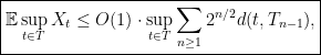
where $(t, A)$ is the distance between the point $X_t$ from the set $A$ , and $\{T_i\}$ is a specific sequence of sets with $T_i\subset T$ . Constructions of these sets will be discussed in a subsequent post.

Continue reading “Bounding the Supremum of a Gaussian Process: Talagrand’s Generic Chaining (Part 1)” →

Spectral Sparsification by Spielman and Srivastava: How They Connected the Dots

In this post, I will discuss my own understanding of the spectral sparsification paper by Daniel Spielman and Nikhil Srivastava (STOC 2008). I will assume the following:

The reader is a beginner, like me, and have already glanced through the Spielman-Srivastava paper (from now on, the SS paper).
The reader has, like me, a basic understanding of spectral sparsification and associated concepts of matrix analysis. I will assume that she has read and understood the Section 2 (Preliminaries) of the SS paper.
The reader holds a copy of the SS paper while reading my post.

First, I will mention the main theorems (actually, I will mention only what they “roughly” say).

Continue reading “Spectral Sparsification by Spielman and Srivastava: How They Connected the Dots” →

Chebyshev’s Inequality

If we have a random variable $X$ and any number $a$ , what is the probability that $X \geq a$ ? If we know the mean of $X$ , Markov’s inequality can give an upper bound on the probability that $X$ . As it turns out, this upper bound is rather loose, and it can be improved if we know the variance of $X$ in addition to its mean. This result is known as Chebyshev’s inequality after the name of the famous mathematician Pafnuty Lvovich Chebyshev. It was first proved by his student Andrey Markov who provided a proof in 1884 in his PhD thesis (see wikipedia).

Continue reading “Chebyshev’s Inequality” →

Markov’s Inequality

How likely is it that the absolute value of a random variable $X$ will be greater than some specific value, say, $a$ ? The Russian mathematician Andrey Andreyevich Markov proved a simple, yet nice, result which enables us to answer the above question.

Markov’s Inequality states that if $X$ is a random variable with mean $\mu$ , and $a>0$ is a positive number, then

$Pr[|X| \geq a] \leq \frac{|\mu|}{a}$

Continue reading “Markov’s Inequality” →